ECSS Miniconference 2022
An Introduction to Probabilistic Programming in Python using PyMC
Danh Phan
Linkedin: @danhpt Twitter: @danhpt
Website: http://danhphan.net
Nov 2022
1. Introduction
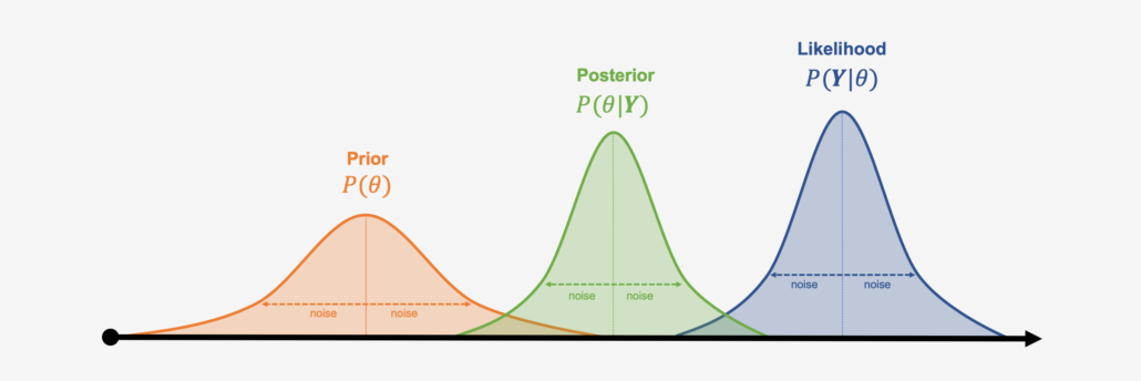
Bayes' Formula
Given two events A and B, the conditional probability of A given that B is true is expressed as follows:
$$P(A|B) = \frac{P(B|A) \times P(A)}{P(B)}$$Bayesian Terminology
Replacing Bayes' Formula with conventional Bayes terms:
$$P(\theta|y) = \frac{P(y|\theta) \times P(\theta)}{P(y)} = \frac{P(y|\theta) \times P(\theta)}{\int P(y|\theta)P(\theta) d\theta}$$The equation expresses how our belief about the value of $\theta$, as expressed by the prior distribution $P(\theta)$ is reallocated following the observation of the data $y$, as expressed by the posterior distribution.

2. Data set
Anscombe's quartet is an interesting group of four data sets that share nearly identical descriptive statistics while in fact having very different underlying relationships between the independent and dependent variables.
plot_data()

3.1. Linear regression
We use the ordinary least squares (OLS) line to fit these data using NumPy's polyfit.
$$y=a*x+b+ε$$
a_ols, b_ols = np.polyfit(x, y, deg=1)
plt.scatter(x, y)
plot_line(a_ols, b_ols,c='r', ls='--', label="Numpy OLS")

3.2. Robust Linear regression
is_outlier = x == 13
a_robust, b_robust = np.polyfit(x[~is_outlier], y[~is_outlier], deg=1)
plt.scatter(x, y);
plot_line(a_ols, b_ols, c='r', ls='--', label="NumPy OLS");
plot_line(a_robust, b_robust, ls='--', label="Robust");

4.1. Bayesian Linear regression
with pm.Model() as ols_model:
    # Priors
    a = pm.Flat("a")
    b = pm.Flat("b")
    σ = pm.HalfFlat("σ")

    # Likelihood
    y_obs = pm.Normal("y_obs", a * x + b, σ, observed=y)

    # MCMC sampling (Default: NUTS)
    ols_trace = pm.sample(2000)
Auto-assigning NUTS sampler...
Initializing NUTS using jitter+adapt_diag...
Multiprocess sampling (4 chains in 4 jobs)
NUTS: [a, b, σ]
Sampling 4 chains for 1_000 tune and 2_000 draw iterations (4_000 + 8_000 draws total) took 6 seconds.
pm.model_to_graphviz(ols_model)
Linear regresion: Numpy vs. PyMC
plt.scatter(x, y);
plot_line(a_ols, b_ols, c='r', ls='--', label="NumPy OLS", lw=3);
plot_line(a_bays, b_bays, c='C0', label="PyMC OLS", lw=2);

Linear regresion: posterior distributions
plt.scatter(x, y);
plot_line(a_ols, b_ols, c='C1', ls='--', label="NumPy OLS", lw=3);
plot_line(a_bays, b_bays, c='C0', label="PyMC OLS", lw=2);
# Plot many lines from posterior distributions
for a_, b_ in (ols_trace.posterior[["a", "b"]].sel(chain=0).thin(100).to_array().T):
    plot_line(a_.values, b_.values, c='C0', alpha=0.2);

Linear regresion: posterior distributions
az.plot_trace(ols_trace);
plt.tight_layout()

4.2. Bayesian Robust Linear regression
with pm.Model() as robust_model:
    # Priors
    a = pm.Normal("a", 0, 2.5)
    b = pm.Normal("b", 0., 10)
    σ = pm.HalfNormal("σ", 2.5)
    ν = pm.Uniform("ν", 1, 10)

    # Likelihood
    y_obs = pm.StudentT("y_obs", mu=a*x + b, sigma=σ, nu=ν, observed=y)

    robust_trace = pm.sample(2000)
Auto-assigning NUTS sampler...
Initializing NUTS using jitter+adapt_diag...
Multiprocess sampling (4 chains in 4 jobs)
NUTS: [a, b, σ, ν]
Sampling 4 chains for 1_000 tune and 2_000 draw iterations (4_000 + 8_000 draws total) took 11 seconds.
pm.model_to_graphviz(robust_model)
Robust Linear regresion: posterior distributions
plt.scatter(x, y);
plot_line(a_robust, b_robust, c='C0', ls='--', label="Robust");
plot_line(a_bays_robust, b_bays_robust, c='C0', label="PyMC OLS", lw=2);
# Plot many lines from posterior distributions
for a_, b_ in (robust_trace.posterior[["a", "b"]].sel(chain=0).thin(100).to_array().T):
    plot_line(a_.values, b_.values, c='C0', alpha=0.2);

Robust Linear regresion: posterior distributions
az.plot_trace(robust_trace);
plt.tight_layout()


References
Theory
- Statistical Rethinking by Richard McElreath
- Statistical Rethinking in PyMC
PyMC
- A Modern Introduction to Probabilistic Programming with PyMC by Austin Rochford
- PyMC quickstart guide, tutorial, and example gallery
- Book: Bayesian Analysis with Python
- Book: Probabilistic Programming & Bayesian Methods for Hackers
- Book: Bayesian Modeling and Computation in Python