PyMCon Web Series
An introduction to multi-output Gaussian processes using PyMC
Danh Phan
Linkedin: @danhpt Twitter: @danhpt
Website: http://danhphan.net
Feb 2023
1. Introduction
We have a training set D, where $$D=\{(x_i,y_i) | i=1,...,N\}$$ where $y_i$ is a scalar output, and $x_i$ is a general input vector.
All input vectors are often aggregated into a matrix $X$, and the output vector $y$ for the output values.
$$X = \begin{bmatrix} x_1 \\ x_2 \\ ... \\ x_N \end{bmatrix} y = \begin{bmatrix} y_1 \\ y_2 \\ ... \\ y_N \end{bmatrix}$$A general model is given by $$y_i = f(x_i,\theta) + \epsilon_i$$ $$ \epsilon_i \sim N(0, \sigma) $$ For simplicity, let's assume $x_i$ is scalar.
1.1 Bayesian Linear Regression
$$f(x_i, \theta) = \beta_0 + \beta_1 x_i$$where $$\theta = [\beta_0, \beta_1]$$ So $$y_i = f(x_i,\theta) + \epsilon_i = \beta_0 + \beta_1 x_i + \epsilon_i$$
The parameter $\theta$ is inferred through Bayes' rule
$$P(\theta|X,y) = \frac{P(y|X,\theta) \times P(\theta)}{P(y|X)} = \frac{P(y|X,\theta) \times P(\theta)}{\int P(y|X,\theta)P(\theta) d\theta} = posterior = \frac{likelihood * prior}{evidence \ or \ marginal \ likelihood} $$Predict unseen data by computing the predictive posterior $$P(y_∗|X_∗,X,y) = \int P(y_∗|\theta, X_∗)P(\theta|𝐗, y)d\theta $$
1.2 Gaussian Process
- The primary goal of the forecasting model is to compute the underlying function $f$ from the noisy observation $y$
- If we less interested in $\theta$, and more interested in model predictive capability => Can infer $f$ directly!
The function $f$ is random and we need to assign a probability distribution over f
Rasmussen and Williams suggested:
*A Gaussian process is a collection of random variables, any finite number of which have a joint Gaussian distribution.*
$$\begin{bmatrix} f(x_i) \\ f(x_j) \\ f(x_k) \\ ... \end{bmatrix} = \mathcal{N}\Bigg(\begin{bmatrix} m(x_i) \\ m(x_j) \\ m(x_k) \\ ... \end{bmatrix}, \begin{bmatrix} k(x_i,x_i) & k(x_i,x_j) & k(x_i,x_k) & ... \\ k(x_j,x_i) & k(x_j,x_j) & k(x_j,x_k) & ... \\ k(x_k,x_i) & k(x_k,x_j) & k(x_k,x_k) & ... \\ ... & ... & ... & ... \end{bmatrix}\Bigg) $$where $m$ and $k$ denote the mean and covariance functions (kernels) respectively. As an alternative way define a function that is distributed according to a Gaussian process as:
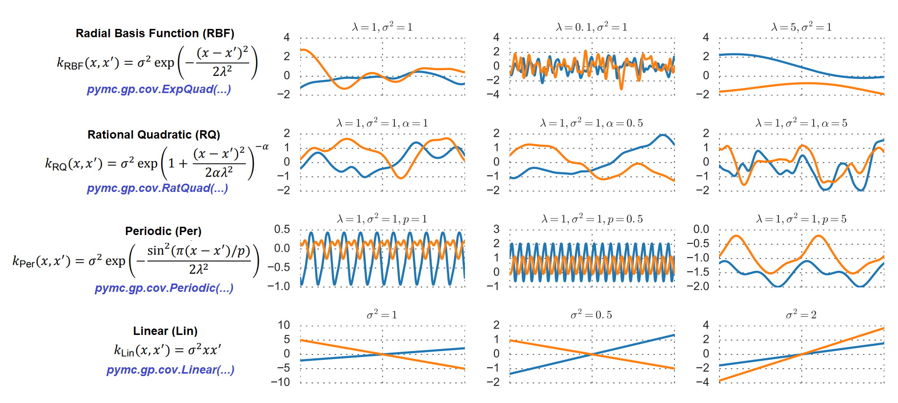
$$f(x) = \mathcal{GP}( m(x), k(x,x') )$$1.3 GP Mean and Covariance Functions
# Data set
data_url = 'https://raw.githubusercontent.com/danhphan/workshops/main/2023-PyMCon/data/salmon.csv'
salmon_data = pd.read_csv(data_url)
x, y = salmon_data[['spawners', 'recruits']].values.T
print("Data shape: ", salmon_data.shape, x.shape, y.shape)
salmon_data.plot.scatter(x='spawners', y='recruits', s=50, figsize=(5,3));
plt.xlabel("x: spawners");
plt.ylabel("y: recruits");
Data shape: (40, 2) (40,) (40,)

2. Model implementation in PyMC
2.1 Bayesian Linear Regression
Simple linear regression: $$y_i = f(x_i,\theta) + \epsilon_i$$ $$ y_i = \beta_0 + \beta_1 x_i + \epsilon_i $$
There are three unknowns, each of which need to be given a prior:
$$\beta_0, \beta_1 \sim \text{Normal}(0, 50)$$$$\sigma \sim \text{HalfNormal}(50)$$# Create a PyMC model
with pm.Model() as linear_salmon_model:
# Prior
beta_0 = pm.Normal('beta_0', mu=0, sigma=50)
beta_1 = pm.Normal('beta_1', mu=0, sigma=50)
sigma = pm.HalfNormal('sigma', sigma=50)
mean = beta_0 + beta_1 * x
# Likelihood
recruits = pm.Normal('recruits', mu=mean, sigma=sigma, observed=y)
# Prior distribution
a_normal_distribution = pm.Normal.dist(mu=0, sigma=50)
plt.hist(pm.draw(a_normal_distribution, draws=1000));

# Prior distribution
a_half_normal_distribution = pm.HalfNormal.dist(sigma=50)
plt.hist(pm.draw(a_half_normal_distribution, draws=1000));

with linear_salmon_model:
    linear_trace = pm.sample(1000, tune=2000, cores=2)
Auto-assigning NUTS sampler...
Initializing NUTS using jitter+adapt_diag...
Multiprocess sampling (2 chains in 2 jobs)
NUTS: [beta_0, beta_1, sigma]
Sampling 2 chains for 2_000 tune and 1_000 draw iterations (4_000 + 2_000 draws total) took 4 seconds.
# Posterior distribution
az.plot_trace(linear_trace.posterior);
plt.tight_layout()

# Prediction
X_pred = np.linspace(0, 500, 100)

ax = salmon_data.plot.scatter(x='spawners', y='recruits', c='k', s=50, figsize=(5,3))
ax.set_ylim(0, None)
for b0,b1 in zip(linear_trace.posterior['beta_0'].sel(chain=0)[:20],
                 linear_trace.posterior['beta_1'].sel(chain=0)[:20]):
    b0,b1=b0.values,b1.values
    ax.plot(X_pred, b0 + b1*X_pred, alpha=0.3, color='seagreen');
plt.xlabel("x: spawners");
plt.ylabel("y: recruits");

2.2 Gaussian Processes in PyMC
$$y_i = f(x_i,\theta) + \epsilon_i$$$$f(x) = \mathcal{GP}(m(x), k(x,x')$$$$f(x) = \mathcal{GP}( Linear, ExpQuad(x,x') )$$with pm.Model() as gp_salmon_model:
ρ = pm.HalfCauchy('ρ', 5)
η = pm.HalfCauchy('η', 5)
M = pm.gp.mean.Linear(coeffs=(salmon_data.recruits/salmon_data.spawners).mean())
K = (η**2) * pm.gp.cov.ExpQuad(input_dim=1, ls=ρ)
σ = pm.HalfNormal('σ', 50)
recruit_gp = pm.gp.Marginal(mean_func=M, cov_func=K)
recruit_gp.marginal_likelihood('recruits',
X=salmon_data.spawners.values.reshape(-1,1),
y=salmon_data.recruits.values, noise=σ)
with gp_salmon_model:
    gp_trace = pm.sample(1000, tune=2000, cores=2, random_seed=42)
Auto-assigning NUTS sampler...
Initializing NUTS using jitter+adapt_diag...
Multiprocess sampling (2 chains in 2 jobs)
NUTS: [ρ, η, σ]
Sampling 2 chains for 2_000 tune and 1_000 draw iterations (4_000 + 2_000 draws total) took 22 seconds.
az.plot_trace(gp_trace, var_names=['ρ', 'η', 'σ']);
plt.tight_layout()

Predict unseen data by computing the predictive posterior $$P(y_∗|X_∗,X,y) = \int P(y_∗|\theta, X_∗)P(\theta|𝐗, y)d\theta $$
$$P(y_∗|X_∗,X,y) = \int P(y_∗|X_∗,f,X)P(f|𝐗,y)df $$# Prediction
with gp_salmon_model:
salmon_pred = recruit_gp.conditional("salmon_pred",
X_pred.reshape(-1,1))
gp_salmon_samples = pm.sample_posterior_predictive(gp_trace,
var_names=['salmon_pred'], random_seed=42)
Sampling: [salmon_pred]
ax = salmon_data.plot.scatter(x='spawners', y='recruits', c='k', s=50)
ax.set_ylim(0, None)
for x in (gp_salmon_samples.posterior_predictive['salmon_pred']
          .sel(chain=0)[:3,:]):
    ax.plot(X_pred, x);

from pymc.gp.util import plot_gp_dist
fig, ax = plt.subplots(figsize=(8,6))
plot_gp_dist(ax, (gp_salmon_samples.posterior_predictive['salmon_pred']
                  .sel(chain=0)[:50,:]), X_pred)
salmon_data.plot.scatter(x='spawners', y='recruits', c='k', s=50, ax=ax)
ax.set_ylim(0, 350);

3. References
- Rasmussen and Williams, 2005. Gaussian Processes for Machine Learning
- Bagas Abisena Swastanto, 2016. Gaussian process regression for long-term time series forecasting
- Chris Fonnesbeck, PyData NYC, 2019. A Primer on Gaussian Processes for Regression Analysis
- Oriol Abril & Bill Engels, PyMC Examples, 2022. PyMC Mean and Covariance Functions
- Notebook codes, Danh Phan, 2023. https://github.com/danhphan/workshops/2023-PyMCon